
Resolution Enhancements – Super Resolution techniques using Deep Learning – Part III
 Image enhancement, picture quality improvement and increasing resolution of images without a significant drop in quality have been one of the major application areas of Deep Learning based Artificial Intelligence techniques in recent years. These technologies are collectively called Super Resolution (SR). This is part III of series of blogs on this topic.
The most basic application of SR related technologies is resolution enhancement. In simple words, we take an image and enlarge it by a multiplying factor such as 2x, 4x or 8x etc. For example, an input image of size 100×200 pixels would be enlarged to 200×400 pixels when performing a 2x enlargement. The goal is to lose as little information as possible when performing such enhancement. Although, there are built-in techniques in almost all popular photo editing applications that try to interpolate the missing pixels using some algorithm when an image is enlarged, the resulting image is usually quite pixelated as the resolution becomes larger. For 4x and larger sizes, the pixelation and other artifacts become quite visible to the naked eye and make the image unusable in any applications requiring large high resolution images.
This is where Deep Learning comes in. With latest Deep Learning techniques, we can build models that learn to produce higher resolution images without significant drop in quality and much reduced pixelation effect compared to standard interpolation techniques used in mainstream software applications.
How it works?
The idea behind SR with Deep Learning is quite simple. In this article we will describe two basic techniques for resolution enhancement:
- Post-upsampling
- Pre-upsampling
Both techniques have pros and cons and we will highlight them as we go along.
Post-upsampling
In this technique, we take an image and first reduce its size by the same factor, to which we want to enlarge it. For example, for a 2x enlargement, we reduce the original image to ½ of its size.
Next we create a Convolutional Neural Network (CNN) (blue rectangles in figure below) composed of convolution filters and layers that process the smaller image and extract features from it as it passes through its layers. For more information on CNNs and how they work, please see excellent tutorial articles here and here.
The feature extraction process may also reduce the image size further, and the output of CNN maybe even a smaller image than ½ in our example. Note that the output is actually not an image any more since it has been transformed into something called feature maps after applying so many convolution filters and should just be called a set of 2-D array or more generally, a tensor of HxWxN where H and W are image height and width and N is the number of channels output by the CNN. This tensor represents the extracted image features and is then passed through an up-sampling network (green rectangle in figure below) to make it larger again, up to the desired size. The final image that comes out at the other end is of the original size (since we reduced it to a fraction of the original size before feeding to the network) .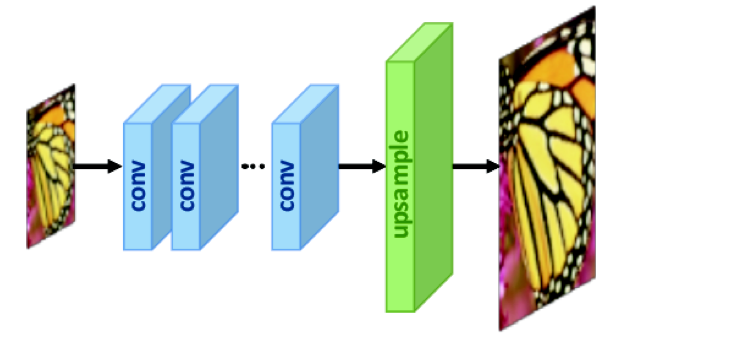
The convolution layers combined with upsampling layers are designed such that when the image comes out at the other end after passing through them, it has been enlarged to the original size. Assuming we were upsampling by a factor of 2x, then the original image was say, size 100×200, we reduced it to 50×100 first, then passed it through our network, and got the output again as 100×200.
Several techniques are used to increase the image size (aka upsampling). The two most commonly used techniques are Transposed Convolutions (aka de-convolutions) and sub-pixel shuffle. Details of these can be found in the given links. There are pros and cons of each technique but they are essentially trying to achieve the same thing. Post-upsampling uses either one, or a mix of the two to scale the image up to the desired size.
Training the Network
Obviously, if we want to enlarge an image, then producing the same image size as the original one doesn’t seem to be very useful in the real world. This is where the model training comes in:
- We feed the network two images, one down-sampled by the same factor as we want to upscale it with e.g. 2x upscaling means down-sampling first by ½ as described above.
- During training, the output of the CNN is compared against the original image. If the output values of pixels are very close to the original, meaning that the network produced a very good replica of the original from a smaller size without losing much information, then it could (in theory) enlarge any given image without giving up significantly on quality.
Pre-upsampling
In this technique, we up-sample the image to the desired size before feeding to the Network. A technique called pixel interpolation is used for this purpose. Pixel interpolation tries to guess the missing pixel values when enlarging an image, since enlargement essentially means generating information that was not there in the original image.
Several interpolation techniques are used for this purpose. Some of them include:
There are other techniques as well with varying degrees of performance for different image types, qualities and categories.
Once the image has been enlarged, it is expected to have some artifacts as a result of interpolation, since it is essentially guess work as to what the values of missing pixels might be if we had an actual image of the larger size of the same scene. The goal of the CNN in this case is to remove those artifacts during training.
Training the Network
The training procedure in this case is as follows:
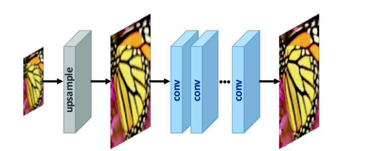
- We create two two images, one of smaller size scaled down by the desired upsampling factor just as before in post-upsampling case
- First the system increases the smaller image’s size to the desired factor using some interpolation method as described above (blinear, bicubic, nearest etc.).
- We feed both images, the upsampled by interpolation, and the original image to the network for training
- The Network (blue rectangles in figure below) is designed in such a way that it maintains the image size as the image passes through it and extracts features and refines it at each convolution layer
- The network trains by comparing the extracted features to the original image
Loss function
For training, we need to set a loss function, that is, the objective function we want our network to minimize. This is usually either pixel wise Mean-Squared-Error (MSE) or L1 loss (direct absolute pixel difference). The network tries to minimize it by adjusting the weights of the CNN filters during training using the well known Gradient Descend algorithm universally used for training Neural Networks. If we are able to minimize this loss function or reduce it to very small value, this means our CNN based model is ready to handle general images and upsample them.
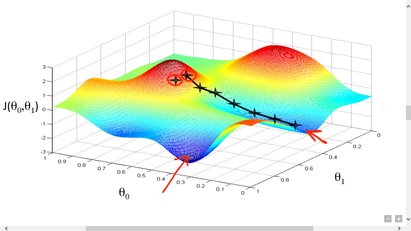
Finding the minimum point of the loss function: Gradient Descend
Please note that we only aim to significantly reduce the loss in real world. We may never find the global minimum point of our loss function. This is because, as we know, the gradient descend algorithm for training a Neural Network searches the minimum point of the loss function by passing all the data (images in our case) in batches through the network again and again, varying weights of the network by a small amount each time and then checking the effect of the variation on the loss function. In other words, its sort of a blind search for minimum point with a rather crude sense of direction of whether we are moving up-hill (away) from the minimum or down-hill (towards it). Gradient descend may very well miss the minimum and then would have to retry catching it again. Learning rate is also a very important hyper-parameter in this regard that let’s the network to update its weights in small increments and gives it a good sense of direction towards the minimum.
Advantages and disadvantages of Post-upsampling
- One of the key advantages of this architecture is that the CNN has to deal with low resolution (smaller sized) images for features extraction since upsampling is only performed at the end. This reduces computational complexity both in terms of memory and computing time.
- The disadvantage is that due to limited capacity of the network, it is unable to learn complex feature interactions within images[Source]
- Another disadvantage is that we need to train separate models for each upscale factor e.g. 2x, 4x, 8x etc. since the upscale layer at the end can only enlarge to one specific size.
- Furthermore, the training time is quite large, usually in the order of days for large upscale factors
Advantages and disadvantages of Pre-upsampling
- One of the main advantages of this architecture is that the upsampling is performed in the beginning by well-known interpolation techniques and the CNN only has to refine the noise and other artifacts introduced by this interpolation process. This reduces training complexity and also training time.
- A key disadvantage is that the CNN has to deal with a large, upscaled image size throughout which increases memory and computation cost [Source]
- Another advantage is that since we upscale upfront, and the network outputs the same dimension tensor as the input image, we don’t need to train separate models for different upscale factors. We can use the same network for all enlargement factors, although large upscale factors are expected to produce more artifacts.
Using the trained model
Once we have a trained model, all we need to do is give it a low resolution image that we want to enlarge. The network would enlarge it by the same factor as it was designed and trained to do, and we would hopefully get back a nice resolution-enhanced image.
PSNR: Assessing the performance of SR Model
Most common measure for performance assessment of an SR model is Peak Signal to Noise Ratio (PSNR). PSNR gives us a rough measure of how well the quality of a processed image (output of the model in our case) is compared to the original image. This is done by comparing the output of SR process by the original image using the PSNR formula. Note that MSE is part of PSNR calculation. However, we usually don’t use PSNR itself as the loss function for training our network and only use it to assess model performance after training. We use either MSE or L1 as the loss to be minimized during training. The actual mathematical reasons are beyond the scope of this article but here we give a simplified, intuitive explanation.
The reason lies in the way Neural Networks operate. It is essential for the loss function to be continuous and easily differentiable. This is because we apply chain rule of differentiation while performing back propagation through the network, a process that is essential part of training. During back propagation, the loss function has to be differentiated with respect to the weights of each layer starting from the last (output) layer of the network, all the way to the first one. We therefore need loss functions whose derivative is defined at all points and is also not too computationally expensive to calculate.
There are other performance measures for applications belonging to SR category that are better in some ways than PSNR. We will discuss some of them in one of our next articles in this series.
Improving SR performance: Data Augmentation
Data augmentation, in the context of Image Processing and Computer Vision is the process of making additional copies of images in our training set. New images are added by transforming the already available images in the dataset in some way, to make more data available for training without actually adding any new images.
The augmented images are copies of the original ones with some transformation applied that does not change the actual image in any substantial way but still provides a different view that may be helpful for training. This usually improves model performance substantially during training since the model sees a more diverse set of images and adapts its weights to reduce loss function on a richer dataset.
Some example transformations relevant in SR scenario are as follows:
- Flipping images horizontally and vertically
- Rotating images through an angle
- Cropping part of image by taking a piece of it from the center or randomly and make it a separate image
- Randomly changing brightness, contrast, hue (color variation) and gamma (luminance) values.
This gives the model more variety to play with and generalize itself better to unseen images.
Conclusion and what’s next
In this article, we introduced the most common use cases and applications of AI techniques for image processing and quality enhancement. We also reviewed two basic techniques for image resolution enhancement: Post-upsampling and Pre-upsampling, and discussed the advantages and disadvantages of each. We also described the common loss functions and the use of PSNR for performance assessment of SR applications.
In the next article in this series, we will review more advanced techniques, especially the ones based on Generative Adversarial Networks, progressive resizing, iterative upsampling and down-sampling and describe their advantages and disadvantages. We will also cover additional loss functions, and also methods to assess performance that are better than PSNR. In the last part of this series, we will get an overview of techniques for handling use cases other than basic image enlargement, such as the ones mentioned in the beginning of this article. Stay tuned!!
About Author
 Farhan Zaidi has over 25 years of experience in Software Architecture, Data Engineering and software development in a variety of languages and technologies. He is skilled in designing data-driven, enterprise-grade software systems, as well as Embedded Systems and Systems Programming. His recently co-founded DreamAI with a vision to apply Deep Learning technology in a variety of domains, with a special focus on Computer Vision for Medical Diagnosis, Natural Language Processing and general Predictive Analytics for business problems.
Leave a Reply
Want to join the discussion?Feel free to contribute!